Installation


The installation procedure is quite simple if you use, highly recommended conda package manager
conda install -c jochym elastic
The above command installs elastic with all dependencies into your current conda environment. If you want to add my anaconda.org channel into your conda installation you need to run following command:
conda config –add channels jochym
The above method has additional benefit of providing current installation of ASE and spglib libraries.
To install the code pedestrian way you need to install following python packages (most, if not all, are available in major linux distributions):
- SciPy and NumPy libraries
- matplotlib (not strictly required, but needed for testing and plotting)
- ASE system
- Some ASE calculator (VASP, GPAW, abinit, ...), but be warned that for now the code was developed using VASP only. I will be happy to help you extending it to other calculators.
- spglib space group library
- pyspglib python space group module
This is highly system-dependent and I am unable to provide detailed support for this type of install - I use conda install of ASE/elastic myself!
Some legacy installation guides which may help you with manual process could be find at the QE-doc project pages.
Testing
All modules have small testing sets at the end. You can run these test by simply running each module as a python script:
python parcalc.py
which will run a short series of single-point calculations on the MgO unit cell and plot the resulting equation of state.
The main module testing routine:
python elastic.py
will run the equation of state and elastic tensor calculations for a set of small crystals - one for each Bravais lattice. This may take some considerable time.
The testing routines will probably not work out of the box in your system. Review the comments at the end of the files to make them work. I will try to make them as setup-agnostic as possible.
Usage
In this section we assume that you have all parts of ASE properly installed and the elastic is installed and working properly. The examples are available in the example subdirectory. The code below use also scipy, numpy and matplotlib functions. The VASP calculator is used in all examples (at least for now).
IPython notebook with additional example presents calculation using QE-util package
Simple Parallel Calculation
Once you have everything installed and running you can run your first real calculation. The testing code at the end of the parcalc.py may be used as an example how to do it. The first step is to import the modules to your program (the examples here use VASP calculator):
from ase.lattice.spacegroup import crystal
from parcalc import ClusterVasp, ParCalculate
import ase.units as units
import numpy
import matplotlib.pyplot as plt
next we need to create the crystal, MgO in this case:
a = 4.194
cryst = crystal(['Mg', 'O'],
                [(0, 0, 0), (0.5, 0.5, 0.5)],
                spacegroup=225,
                cellpar=[a, a, a, 90, 90, 90])
We need a calculator for our job, here we use VASP and ClusterVasp defined in the parcalc module. You can probably replace this calculator by any other ASE calculator but this was not tested yet. Thus let us define the calculator:
# Create the calculator running on one, eight-core node.
# This is specific to the setup on my cluster.
# You have to adapt this part to your environment
calc = ClusterVasp(nodes=1, ppn=8)

# Assign the calculator to the crystal
cryst.set_calculator(calc)

# Set the calculation parameters
calc.set(prec = 'Accurate', xc = 'PBE', lreal = False,
            nsw=30, ediff=1e-8, ibrion=2, kpts=[3,3,3])

# Set the calculation mode first.
# Full structure optimization in this case.
# Not all calculators have this type of internal minimizer!
calc.set(isif=3)
Finally, run our first calculation. Obtain relaxed structure and residual pressure after optimization:
print "Residual pressure: %.3f bar" % (
            cryst.get_isotropic_pressure(cryst.get_stress()))
If this returns proper pressure (close to zero) we can use the obtained structure for further calculations. For example we can scan the volume axis to obtain points for equation of state fitting. This will demonstrate the ability to run several calculations in parallel - if you have a cluster of machines at your disposal this will speed up the calculation considerably:
# Lets extract optimized lattice constant.
# MgO is cubic so a is a first diagonal element of lattice matrix
a=cryst.get_cell()[0,0]

# Clean up the directory
calc.clean()

sys=[]
# Iterate over lattice constant in the +/-5% range
for av in numpy.linspace(a*0.95,a*1.05,5):
    sys.append(crystal(['Mg', 'O'], [(0, 0, 0), (0.5, 0.5, 0.5)],
                spacegroup=225, cellpar=[av, av, av, 90, 90, 90]))

# Define the template calculator for this run
# We can use the calc from above. It is only used as a template.
# Just change the params to fix the cell volume
calc.set(isif=2)

# Run the calculation for all systems in sys in parallel
# The result will be returned as list of systems res
res=ParCalculate(sys,calc)

# Collect the results
v=[]
p=[]
for s in res :
    v.append(s.get_volume())
    p.append(s.get_isotropic_pressure(s.get_stress()))

# Plot the result (you need matplotlib for this
plt.plot(v,p,'o')
plt.show()
If you set up everything correctly you should obtain plot similar to this:
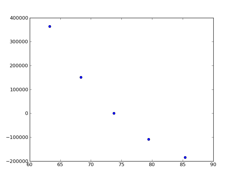
The pressure dependence on volume in MgO crystal (example1.py).
Birch-Murnaghan Equation of State
Let us now use the tools provided by the modules to calculate equation of state for the crystal and verify it by plotting the data points against fitted EOS curve. The EOS used by the module is a well established Birch-Murnaghan formula (P - pressure, V - volume, B - parameters):
We will start with the same crystal optimized above, but this time we will use a new functionality imported from the elastic module. This module acts as a plug-in for the Atoms class - extending their range of quantities accessible for the user:
import elastic
from elastic import BMEOS

a = 4.194
cryst = crystal(['Mg', 'O'],
                [(0, 0, 0), (0.5, 0.5, 0.5)],
                spacegroup=225,
                cellpar=[a, a, a, 90, 90, 90])
Now we repeat the setup and optimization procedure from the example 1 above but using a new Crystal class (see above we skip this part for brevity). Then comes a new part (IDOF - Internal Degrees of Freedom):
# Switch to cell shape+IDOF optimizer
calc.set(isif=4)

# Calculate few volumes and fit B-M EOS to the result
# Use +/-3% volume deformation and 5 data points
fit=cryst.get_BM_EOS(n=5,lo=0.97,hi=1.03)

# Get the P(V) data points just calculated
pv=numpy.array(cryst.pv)

# Sort data on the first column (V)
pv=pv[pv[:,0].argsort()]

# Print just fitted parameters
print "V0=%.3f A^3 ; B0=%.2f GPa ; B0'=%.3f ; a0=%.5f A" % (
        fit[0], fit[1]/units.GPa, fit[2], pow(fit[0],1./3))

v0=fit[0]

# B-M EOS for plotting
fitfunc = lambda p, x: [BMEOS(xv,p[0],p[1],p[2]) for xv in x]

# Ranges - the ordering in pv is not guarateed at all!
# In fact it may be purely random.
x=numpy.array([min(pv[:,0]),max(pv[:,0])])
y=numpy.array([min(pv[:,1]),max(pv[:,1])])


# Plot the P(V) curves and points for the crystal
# Plot the points
plt.plot(pv[:,0]/v0,pv[:,1],'o')

# Mark the center P=0 V=V0
plt.axvline(1,ls='--')
plt.axhline(0,ls='--')

# Plot the fitted B-M EOS through the points
xa=numpy.linspace(x[0],x[-1],20)
plt.plot(xa/v0,fitfunc(fit,xa),'-')
plt.draw()
If you set up everything correctly you should obtain fitted parameters printed out in the output close to:
and the following (or similar) plot:
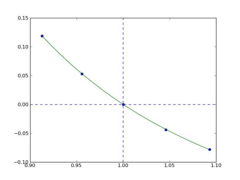
The pressure dependence on volume in MgO crystal (example2.py).
Calculation of the elastic tensor
Finally let us calculate an elastic tensor for the same simple cubic crystal - magnesium oxide (MgO). For this we need to create the crystal and optimize its structure (see Simple Parallel Calculation above). Once we have an optimized structure we can switch the calculator to internal degrees of freedom optimization (IDOF) and calculate the elastic tensor:
# Switch to IDOF optimizer
calc.set(isif=2)

# Elastic tensor by internal routine
Cij, Bij=cryst.get_elastic_tensor(n=5,d=0.33)
print "Cij (GPa):", Cij/units.GPa
To make sure we are getting the correct answer let us make the calculation for \(C_{11}, C{12}\) by hand. We will deform the cell along a (x) axis by +/-0.2% and fit the 3:math:^{rd} order polynomial to the stress-strain data. The linear component of the fit is the element of the elastic tensor:
# Create 10 deformation points on the a axis
sys=[]
for d in linspace(-0.2,0.2,10):
    sys.append(cryst.get_cart_deformed_cell(axis=0,size=d))

# Calculate the systems and collect the stress tensor for each system
r=ParCalculate(sys,cryst.calc)
ss=[]
for s in r:
    ss.append([s.get_strain(cryst), s.get_stress()])

# Plot strain-stress relation
ss=[]
for p in r:
    ss.append([p.get_strain(cryst),p.get_stress()])
ss=array(ss)
lo=min(ss[:,0,0])
hi=max(ss[:,0,0])
mi=(lo+hi)/2
wi=(hi-lo)/2
xa=linspace(mi-1.1*wi,mi+1.1*wi, 50)
plt.plot(ss[:,0,0],ss[:,1,0],'k.')
plt.plot(ss[:,0,0],ss[:,1,1],'r.')

plt.axvline(0,ls='--')
plt.axhline(0,ls='--')

# Now fit the polynomials to the data to get elastic constants
# C11 component
f=numpy.polyfit(ss[:,0,0],ss[:,1,0],3)
c11=f[-2]/units.GPa

# Plot the fitted function
plt.plot(xa,numpy.polyval(f,xa),'b-')

# C12 component
f=numpy.polyfit(ss[:,0,0],ss[:,1,1],3)
c12=f[-2]/units.GPa

# Plot the fitted function
plt.plot(xa,numpy.polyval(f,xa),'g-')

# Here are the results. They should agree with the results
# of the internal routine.
print 'C11 = %.3f GPa, C12 = %.3f GPa => K= %.3f GPa' % (
        c11, c12, (c11+2*c12)/3)

plt.show()
If you set up everything correctly you should obtain fitted parameters printed out in the output close to:
\(C_{ij}\) (GPa): [ 319.1067 88.8528 139.35852632]
With the following result of fitting:
\(C_{11}\) = 317.958 GPa, \(C_{12}\) = 68.878 GPa => K= 151.905 GPa
and the following (or similar) plot:
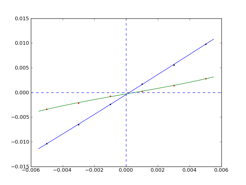
The pressure dependence on volume in MgO crystal (example3.py).